Convex combination

Visualization of convex combinations of order 1, 2 and 3 in Geogebra

Convex Combination in 3D with 4 Vectors

Introduction

In convex geometry, a convex combination is a linear combination of points (which can be vectors, scalars, or more generally points in an affine space) where all coefficients are non-negative and sum to 1. ^[1]

Definition - Convex Combination

More formally, given a finite number of points $x_{1}, x_{2}, \dots, x_{n}$ in a real vector space, a convex combination of these points is a point of the form

λ_{1} x_{1} + λ_{2} x_{2} + \dots + λ_{n} x_{n}

where the real numbers $λ_{i}$ satisfy $λ_{i} \geq 0$ and $λ_{1} + λ_{2} + \dots + λ_{n} = 1 .$ ^[1]

Remark - outside of convex hull

In the animation of the tetrahedron there are examples of points that

fulfill $λ_{1} + λ_{2} + \dots + λ_{n} = 1$ , but
violate the condition $λ_{i} \geq 0$ .

In case that on $λ_{i}$ is negative, then linear combination

λ_{1} x_{1} + λ_{2} x_{2} + \dots + λ_{n} x_{n}

is a point outside the tetrahedron (see animation and consider, when values become negative.

Convex combinations in the plane

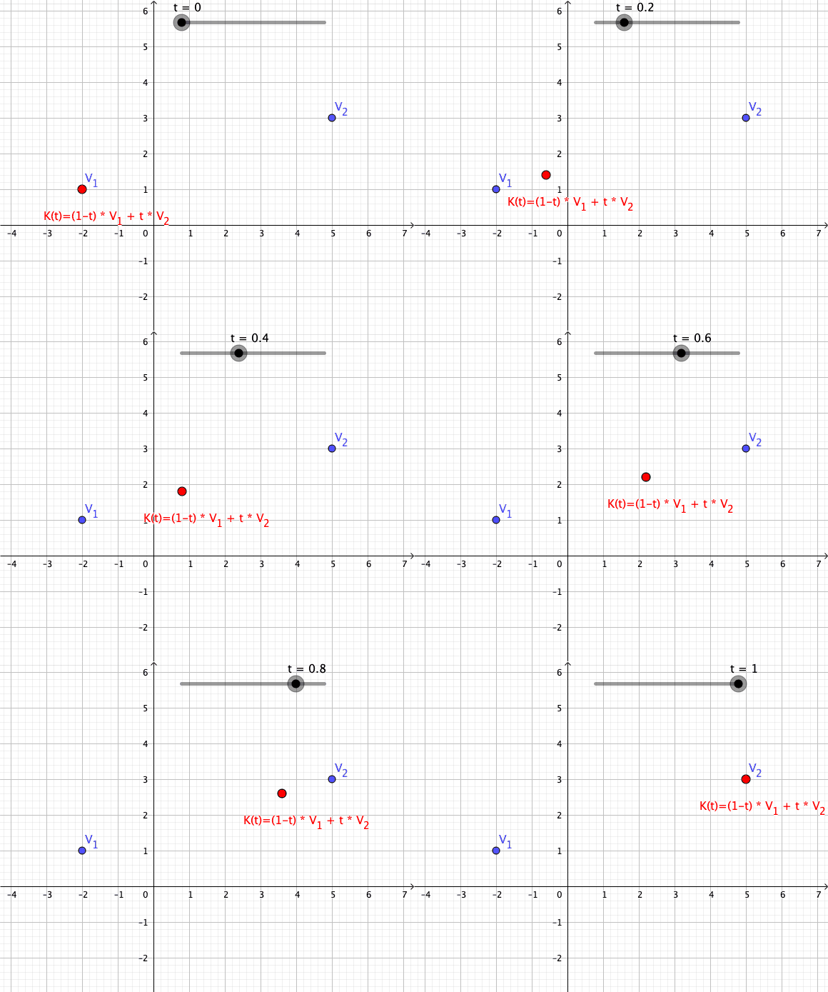
If we consider a convex combinations in the plane, then the underlying vector space is the two-dimensional space $V : = ℝ^{2}$ . First, we consider convex combinations of two vectors in $ℝ^{2}$ . Later we transfer that to infinite dimensional vector spaces of functions and visualize convex combination as GIF animation with Open Source Geogebra. By the condition $λ_{1} + λ_{2} = 1$ , scalars are interdependent. For example, if we define $t \in [0, 1]$ , then we can set $λ_{1} : = (1 - t)$ and $λ_{2} : = t$ .

Convex combinations as mappings into the vector space

File:Convex combination 1 ord with geogebra.gif

Convex combination of two points as GIF-Animation - generated with geogebra

Convex combination of two functions

Geogebra: Interaktives Applet - Download: Geogebra-File

Convex Combination as a Mapping

Now we consider the convex combination as a mapping $K : [0, 1] \to V$ into the underlying vector space. Due to the fact that the equation can generally represent 1st order convex combinations of 2 vectors $v_{1}, v_{2} \in V$ as follows over the mapping $K$ :

K (t) : = (1 - t) \cdot v_{1} + t \cdot v_{2}

Convex Combination of 2 Points

As a particular example, every convex combination of two points lies on the line segment between the points.^[1]

Convex Combination of 2 Functions as Vectors

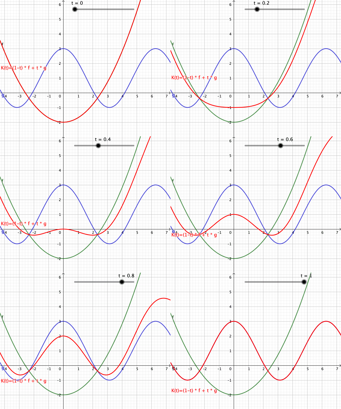
Let $[a, b] = [4, 7]$ be an interval and as the first function is defined as a polynomial $f : [a, b] \to ℝ$ .

f (x) : = \frac{3}{10} \cdot x^{2} - 2

As the second function a trigonometric function $g : [a, b] \to ℝ$ was chosen for the convex combination in the vector space of continuous functions.

g (x) : = 2 \cdot c o s (x) + 1

The animation above illustrates the convex combination $K (t) : = (1 - t) \cdot f + t \cdot g$ .

Remark - Vector space of continuous functions

Both functions $f, g$ and $K (t)$ for all $t \in [0, 1]$ are elements of the vector space of continuous functions from $[a, b]$ to $ℝ$ (i.e. $f, g, K (t) \in 𝒞 ([a, b], ℝ)$ ).

Remark - Deformation

If the first function $f$ describes the initial shape and $g$ the target shape. A convex combinations of those functions can describe (e.g. in computer graphics) a continuous deformation of an initial shape into a target shape.

Convex combination of more than 2 Points

The figure above, the point $P$ is a convex combination of the three points, while $Q$ is not. ( $Q$ is however an affine combination of the three points, as their affine hull is the entire plane.)]]

Convex combination of n points

A set is convex if it contains all convex combinations of its points. The convex hull of a given set of points is identical to the set of all their convex combinations.^[1]

\begin{matrix} v & = & λ_{1} v_{1} + λ_{2} v_{2} + \dots + λ_{n} v_{n} \\ = & \sum_{i = 1}^{n} λ_{i} v_{i}, \\ mit & 0 \leq λ_{i} \leq 1, \sum_{i = 1}^{n} λ_{i} = 1 . \end{matrix}

Linear Combinations and Convex Combinations

There exist subsets of a vector space that are not closed under linear combinations but are closed under convex combinations. For example, the interval $[0, 1]$ is convex but generates the real-number line under linear combinations. Another example is the convex set of probability distributions, as linear combinations preserve neither non-negativity nor affinity (i.e., having total integral one).

Convex combinations of convex combinations

In the animation above you can see a convex combination of 2 vectors in the plane or in a function space. If one uses three points then one can create a 1st order convex combination between every two points. We will now consider higher order convex combinations by constructing e.g. a 2nd order convex combination generated from two 1st order convex combinations. Generally from 2 convex combinations of order $n$ you can create a convex combination of order $n + 1$ .

Convex hull

The set of all convex combinations of a given set of vectors is called a convex hull (see also p-convex hull).

Video convex combinations in the plane

File:Convex combination geogebra.webm

Geogebra: Interactive applet - Download:' Geogebra-File

Remarks video about convex combinations of order 1, 2 and 3 in Geogebra

In the video you can see convex combinations of the

1st order between $A_{1}$ and $B_{1}$ without auxiliary points,
2nd order between $A_{2}$ and $B_{2}$ with auxiliary point $S_{1}$ ,
3rd order between $A_{3}$ and $B_{3}$ with auxiliary points $H_{1}, H_{2}$ ,

Convex combinations as polynomials of t

Convex combinations can be conceived as polynomials where the coefficients come from a vector space $(V, +, \cdot, ℝ)$ (see also Polynomial Algebra). For example, if one chooses $V : = ℝ^{n}$ , one can take a convex combination $K$ to be an element of algebra of polynomial $V [t]$ .

3D convex combination - 1st order

For example, choosing $n = 3$ and $V : = ℝ^{3}$ , a 1st order convex combination is defined as follows.

A = (\begin{matrix} 1 \\ 2 \\ 4 \end{matrix}), B = (\begin{matrix} 4 \\ 1 \\ 0 \end{matrix}), K (t) : = (1 - t) \cdot A + t \cdot B = (B - A) \cdot t + A

Thus, a 1st order convex combination yields a polynomial of degree 1. with argument $t$ . Represent the convex combination in Geogebra 3D with $t \in [0, 1]$ (see also Representation of a Straight Line by Direction Vector and Location Vector).

3D convex combination - 2nd order

Choosing again $n = 3$ and $V : = ℝ^{3}$ with an auxiliary point $H_{1} \in V$ , two 1st order convex combinations yield 2nd order convex combinations.

H_{1} = (\begin{matrix} 2 \\ 2 \\ 2 \end{matrix}), \begin{matrix} K_{(1, 1)} (t) & : = & (H_{1} - A) \cdot t + A \\ K_{(1, 2)} (t) & : = & (B - H_{1}) \cdot t + H_{1} \\ K_{2} (t) & : = & ((H_{1} - A) \cdot t + A) \cdot (1 - t) + ((B - H_{1}) \cdot t + H_{1}) \cdot t \end{matrix}

Represent $K_{2}$ as a polynomial $K_{2} (t) = P_{2} \cdot t^{2} + P_{1} \cdot t^{1} + P_{0} \cdot t^{0}$ and calculate for $n = 2$ ( $n = 3, 4, . . .$ ) the coefficients in $P_{k} \in V = ℝ^{3}$ .

Bernstein polynomial - order 1

\begin{matrix} K_{1} (t) & : = & A \cdot (1 - t) + B \cdot t \\ = & A \cdot (1 - t)^{1} \cdot t^{0} + B \cdot (1 - t)^{0} \cdot t^{1} \end{matrix}

Calculation of the polynomial - order 2

\begin{matrix} K_{2} (t) & : = & ((H_{1} - A) \cdot t + A) \cdot (1 - t) + ((B - H_{1}) \cdot t + H_{1}) \cdot t \\ = & (H_{1} \cdot t - A \cdot t + A) - (H_{1} \cdot t^{2} - A \cdot t^{2} + A \cdot t) \\ + (B \cdot t^{2} - H_{1} \cdot t^{2} + H_{1} \cdot t) \\ = & (B - H_{1} + A) \cdot t^{2} + 2 \cdot (H_{1} - A) \cdot t + A \end{matrix}

Bernstein polynomial - order 2

\begin{matrix} K_{2} (t) & : = & ((H_{1} - A) \cdot t + A) \cdot (1 - t) + ((B - H_{1}) \cdot t + H_{1}) \cdot t \\ = & A \cdot (1 - t)^{2} + 2 \cdot H_{1} \cdot t \cdot (1 - t) + B \cdot t^{2} \end{matrix}

Bernstein polynomial - order 3

\begin{matrix} K_{3} (t) & : = & A \cdot (1 - t)^{3} + 3 \cdot H_{1} \cdot (1 - t)^{2} \cdot t + 3 \cdot H_{2} \cdot (1 - t) \cdot t^{2} + B \cdot t^{3} \end{matrix}

Convex combination as a mapping

A convex combination can be used to interpolate points $A = v_{1}$ and $B = v_{n}$ . Furthermore, if the auxiliary points $H_{1} = v_{2}$ ,.... $H_{n_{1}} = v_{n - 1}$ are given for a convex combination $n$ -th order. The convex combinations can be generally thought of as mapping from the interval $[0, 1]$ to $ℝ^{n}$ as follows:

\begin{matrix} K_{n} : & [0, 1] & \to & ℝ^{n} \\ t & \mapsto & \sum_{k = 0}^{n} (\binom{n}{k}) (1 - t)^{n - k} \cdot t^{k} \cdot v_{k + 1} \\ = (\binom{n}{0}) (1 - t)^{n} v_{1} + (\binom{n}{1}) (1 - t)^{n - 1} t v_{2} + \dots + (\binom{n}{n}) t^{n} v_{n} \end{matrix}

Interpolations

Convex combinations can also be used to interpolate polynomials. Start first with first order interpolations by interpolating the points with straight lines of the form $f_{k} (x) : = m_{k} \cdot x + b_{k}$ . Here, the points $𝔻 : = {(x_{0}, y_{0}), \dots, (x_{n}, y_{n})}$ are given data points that are interpolated piecewise using the functions $f_{k} (x) : = m_{k} \cdot x + b_{k}$ . Compute from the convex combinations $P_{k} (t) \in ℝ^{2}$ the functional representation $f_{k} : [x_{k - 1}, x_{k}] \to ℝ$ with $f_{k} (x) : = m_{k} \cdot x + b_{k}$ :

P_{k} (t) : = (1 - t) \cdot (\begin{matrix} x_{k - 1} \\ y_{k - 1} \end{matrix}) + t \cdot (\begin{matrix} x_{k} \\ y_{k} \end{matrix})

Calculation of t as a function of x

Given $x \in [x_{k - 1}, x_{k}] \subset ℝ$ . We now compute the corresponding $t \in [0, 1]$ for the convex combination with the preliminary consideration that $t = 0$ for $x = x_{k - 1}$ and $t = 1$ for $x = x_{k}$ . The following figure takes the linear transformation $T : [x_{k - 1}, x_{k}] \to [0, 1]$ .

T (x) : = \frac{x - x_{k - 1}}{x_{k} - x_{k - 1}}

Calculation of the function value at x

The convex combination

P_{k} (t) : = (1 - t) \cdot (\begin{matrix} x_{k - 1} \\ y_{k - 1} \end{matrix}) + t \cdot (\begin{matrix} x_{k} \\ y_{k} \end{matrix})

gives the interpolation point of the graph. However, we only need the y-coordinate of the corresponding interpolation point $P_{k} (t) = (\begin{matrix} (1 - t) \cdot x_{k - 1} + t \cdot x_{k} \\ (1 - t) \cdot y_{k - 1} + t \cdot y_{k} \end{matrix})$ . So we use the following term: $(1 - t) \cdot y_{k - 1} + t \cdot y_{k}$ .

Functional representation

Substituting for $t \in [0, 1]$ gives the linear interpolation function $f_{k} : [x_{k - 1}, x_{k}] \to ℝ$ over:

f_{k} (x) : = (1 - \underset{= t}{\underset{⏟}{\frac{x - x_{k - 1}}{x_{k} - x_{k - 1}}}}) \cdot y_{k - 1} + (\underset{= t}{\underset{⏟}{\frac{x - x_{k - 1}}{x_{k} - x_{k - 1}}}}) \cdot y_{k}

.

Learning Tasks

Calculate the coefficients $m_{k}, b_{k} \in ℝ$ of the function $f_{k} : [x_{k - 1}, x_{k}] \to ℝ$ with $f_{k} (x) : = m_{k} \cdot x + b_{k}$ !
Transfer this interpolation to convex combination of order 3 and consider how, depending on the data points, you must choose the two auxiliary points of the interpolation so that the interpolation is differentiable and generates differentiable transitions between the interpolation points in the plot.
What geometric properties must auxiliary points between two adjacent interpolation intervals have for differentiability.

Interpolation with convex combination of order 3

Geogebra: Interactive Applet - Download: Geogebra-File

Develop a mathematical/algebraic description by terms for the following:

The green stippled lines are 1st order convex combinations,
At the vertices of the open Polygon course, create an angle bisector (constructively, this can be implemented by a rhombus, where two sides and a vertex are defined by two adjacent lines in the polygon course).
Create an orthogonal through the connection point of two adjacent lines in the polygon course.
Analyze the figure above and determine the next steps for defining the two auxiliary points for a 3rd order convex combination. The procedure is not clear especially at the boundary points of the polygon course. What speaks to your choice of mathematical implementation?

Use altogether methods from linear algebra (e.g. scalar product,... for the vectorial description of the above geometric procedure.

Morphing and the use of convex combinations

In the following section we will consider transformations of images in the context of convex combinations. In Morphing there are different mathematical tools. Here we will only consider aspects in the context of convex combinations.

Error creating thumbnail:

Look at the above GIF animation and first take two different black and white images transform the first image pixel by pixel to the second image by applying a convex combination from gray level values (black=0,...255=white) of a pixel in image 1 to a pixel in image 2 (implementation e.g. in Octave Image Processing v7.3.0 or Octave Image Processing v5.2.0. Note that the convex combinations yields real values of brightness in the gray levels, which must rounded to integer values (e.g. 232.423 to 232 = approximately white). This is necessary due to that the fact that brightness encoding is done with 256 values (Byte).
Transfer the procedure to color images only, similarly transferring color values for the primary colors from grayscale values to color values.
In the above morphing animation, however, not only static pixel-by-pixel convex combinations are made, but for fixedly defined points, such as eyes, a spatial transformation process also takes place. Consider how, for example, the center of the iris in the eye is spatially shifted from image1 to image2.
now connect spatial transformation processes with a color adjustment of the pixels, so that a pixel moves from the location $(x_{1}, y_{1})$ in the image matrix to $(x_{2}, y_{2})$ and on the way from $(x_{1}, y_{1})$ to $(x_{2}, y_{2})$ the color changes from yellow to blue.

CAS4Wiki

With the following CAS4Wiki commands you can play around with the definition of curves in $ℝ^{2}$

Curves in $ℝ^{2}$ and $ℝ^{3}$