Multiple linear regression

Template:RoundBoxTop Template:Tertiary Template:Notes This learning resource summarises the main teaching points about multiple linear regression (MLR), including key concepts, principles, assumptions, and how to conduct and interpret MLR analyses.

Prerequisites:

1. Correlation
2. Linear regression

What is MLR?

• Multiple linear regression (MLR) is a multivariate statistical technique for examining the linear correlations between two or more independent variables (IVs) and a single dependent variable (DV).
• Research questions suitable for MLR can be of the form "To what extent do X1, X2, and X3 (IVs) predict Y (DV)?"
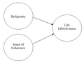
  e.g., "To what extent does people's age and gender (IVs) predict their levels of blood cholesterol (DV)?"
• MLR analyses can be visualised as path diagrams and/or venn diagrams

• MLR studies the relation between two or more IVs and a single DV.
  MLR studies the relation between two or more IVs and a single DV.
• MLR is used to statistically 'distill' the relative contribution of two or more IVs on a single DV.
  MLR is used to statistically 'distill' the relative contribution of two or more IVs on a single DV.
• What other ways can you think of to explain the purpose of MLR?
  What other ways can you think of to explain the purpose of MLR?

Results

• MLR analyses produce several diagnostic and outcome statistics which are summarised below and are important to understand.
• Make sure that you can learn how to find and interpret these statistics from statistical software output.

Correlations

Examine the linear correlations between (usually as a correlation matrix, but also view the scatterplots):

• IVs
• each IV and the DV
• DVs (if there is more than 1)

Effect sizes

R

1. (Big) R is the multiple correlation coefficient for the relationship between the predictor and outcome variables.
2. Interpretation is similar to that for little r (the linear correlation between two variables), however R can only range from 0 to 1, with 0 indicating no relationship and 1 a perfect relationship. Large values of R indicate more variance explained in the DV.
3. R can be squared and interpreted as for r², with a rough rule of thumb being .1 (small), .3 (medium), and .5 (large). These R² values would indicate 10%, 30%, and 50% of the variance in the DV explained respectively.
4. When generalising findings to the population, the R² for a sample tends to overestimate the R² of the population. Thus, adjusted R² is recommended when generalising from a sample, and this value will be adjusted downward based on the sample size; the smaller the sample size, the greater the reduction.
5. The statistical significance of R can be examined using an F test and its corresponding p level.
6. Reporting example: R² = .32, F(6, 217) = 19.50, p = .001
   1. "6, 217" refers to the degrees of freedom - for more information, see about half-down this page

Cohen's ƒ²

• Cohen's ƒ² is based on the R² and is an alternate indicator of effect size for MLR.

Coefficients

An MLR analysis produces several useful statistics about each of the predictors. These regression coefficients are usually presented in a Results table (example) which may include:

• Constant (or Intercept) - the starting value for DV when the IVs are 0
• B (unstandardised) - used for building a prediction equation
• Confidence intervals for B - the probable range of population values for the Bs
• β (standardised) - the direction and relative strength of the predictors on a scale ranging from -1 to 1
• Zero-order correlation (r) - the correlation between a predictor and the outcome variable
• Partial correlations (pr) - the unique correlations between each IV and the DV (i.e., without the influence of other IVs) (labelled "partial" in SPSS output)
• Semi-partial correlations (sr) - similar to partial correlations (labelled "part" in SPSS output); squaring this value provides the percentage of variance in the DV uniquely explained by each IV (sr²)
• t, p - indicates the statistical significance of each predictor. Degrees of freedom for t is n - p - 1.

Equation

• A prediction equation can be derived from the regression coefficients in a MLR analysis.
• The equation is of the form
  

$\hat{Y}=bx+a$ (for predicted values) or
$Y=bx+a+e$ (for observed values)

Residuals

A residual is the difference between the actual value of a DV and its predicted value. Each case will have a residual for each MLR analysis. Three key assumptions can be tested using plots of residuals:

1. Linearity: IVs are linearly related to DV
2. Normality of residuals
3. Equal variances (Homoscedasticity)

Power

• Post-hoc statistical power calculator for MLR (danielsoper.com)

Advanced concepts

• Partial correlations
• Use of hierarchical regression to partial out or remove the effect of 'control' variables
• Interactions between IVs
• Moderation and mediation

Writing up

When writing up the results of an MLR, consider describing:

• Assumptions: How were they tested? To what extent were the assumptions met?
• Correlations: What are they? Consider correlations between the IVs and the DV separately to the correlations between the IVs.
• Regression coefficients: Report a table and interpret
• Causality: Be aware of the limitations of the analysis - it may be consistent with a causal relationship, but it is unlikely to prove causality
• See also: Sample write-ups

FAQ

What if there are univariate outliers?

Basically, explore and consider what the implications might be - do these "outliers" impact on the assumptions? A lot depends on how "outliers" are defined. It is probably better to consider distributions in terms of the shape of the histogram and skewness and kurtosis, and whether these values are unduely impacting on the estimates of linear relations between variables. In other words, what are the implications? Ultimately, the researcher needs to decide whether the outliers are so severe that they are unduely influencing results of analyses or whether they are relatively benign. If unsure, explore, test, try the analyses with and without these values etc. If still unsure, be conservative and remove the data points or recode the data.

See also

• Tutorials/Activities
  • Life expectancy MLR activity
  • MLR quiz (Practice)
  • MLR data analysis tutorial
• Lectures
  • Multiple linear regression I
  • Multiple linear regression II
• Other
  • Four assumptions of multiple regression that researchers should always test (Osborne & Waters, 2002)
  • Least-Squares Fitting
  • Logistic regression
  • Multiple linear regression (Commons)

References

1. Allen & Bennett 13.3.2.1 Assumptions (pp. 178-179)
2. Francis 5.1.4 Practical Issues and Assumptions (pp. 126-128)
3. Green, S. B. (1991). How many subjects does it take to do a regression analysis?. Multivariate Behavioral Research, 26, 499-510.
4. Knofczynski, G. T., & Mundfrom, D. (2008). Sample sizes when using multiple linear regression for prediction. Educational and Psychological Measurement, 68, 431-442.
5. Wilson Van Voorhis, C. R. & Morgan, B. L. (2007). Understanding power and rules of thumb for determining sample sizes. Tutorials in Quantitative Methods for Psychology, 3(2), 43-50.

External links

• Correlation and simple least squares regression (Zady, 2000)
• Multiple regression (Statsoft)
• Multiple regression assumptions (ERIC Digest)